The use of Logistic Regression to study individual determinants of crime risk at the City of Buenos Aires [1]

by Alejandra Otamendi, November 2011

I. Introduction

As part of a national study on crime and violence inArgentina, we analyzed the National Survey of Risk Factors of 2009 (ENFR) conducted by the National Ministry of Health. The objective of this study was to identify which individual characteristics of the population increase the chances of being a victim of armed robbery in the City ofBuenos Airesin 2009.

Since the dependent variable (being robbed) is a dichotomous one, we conducted a logistic regression model. From a set of different variables, we decided to include those that were theoretically relevant or that were useful predictors of individual robbery in previous studies and of course, those that were included in the survey. These variables were: sex, age group, last level of education completed (as a proxy of social position) and having witnessed a robbery occurring to others. Since all of them were also categorical variables, we created dummy variables to include them in the model.

In the following lines, we will show you how we proceeded and finally the doubts that we have and that you may be able to answer or at least to give us your opinion.

II. Main steps and results

First of all, we decided which variables to include as individual predictors of armed robbery in Buenos Aires. Since they were categorical, we created dummy variables as follows:

Codifications of categorical variables

After conducting the logistic regression with SPSS, we obtained the following results. First, the bus tests show a Chi Squaretest that evaluates the null hypothesis that states that the coefficients (ß) of all the terms (except the constant) included in the model are zero. The Chi Squarefor this contrast is the difference between the value of -2LL for the model only with the constant and the value of -2LL for the current model [2]. Provided that all the tests are significant (p =.000) it shows us that the variables included improved significantly the fit of the model compared to the original one.

  Bus tests of the coefficients of the model

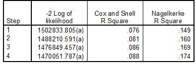
Second, the summary table of the models allows us to evaluate its validity as a whole. In the first column, the smaller the -2LL of the model is, the better its adjustment to the information provided, thus -2LL is sometimes known as a form of “deviation”. In this case it is big because we are working with a large sample of cases. However, what we care at this point is that in the last model the value decreases respect to the previous ones, showing that the last one has the best adjustment of all of them.

Summary of Models

(a) The estimation has finished in the number of iteration 5 because the estimations of the parameters have changed in less than .001.

In the second column, “the R Square of Cox and Snell is a general coefficient of determination used to estimate the proportion of variance of the dependent variable explained by the predictors (independent variables). The R squareof Coxand Snell is based on the comparison of the log of likelihood (LL) for the model with regard to the log of the likelihood (LL) for a model of line base. Its values range between 0 and 1.”[3] In our case it is a low value (0.088) what indicates that only 8.8% of the variation of the dependent variable is explained by the variables included in the model.

In the third column, the R Square of Nagelkerke that is an adjusted version of the RsquareofCoxand Snell, since unlike this one it can cover the full range from 0 to 1, it shows that the model explains 17.4% of the variability. Since this value is still very low, it indicates that we need to include another type of variables to understand more the phenomenon.

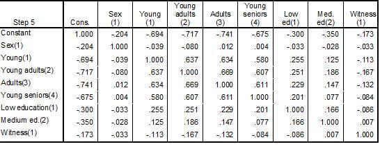
Third, although it comes afterwards, we included the correlation matrix now. From this matrix, we notice that there is no strong correlation between the variables, so all of them can be included.

Correlations Matrix                                                                                                                       Finally, we show only the last step with all the variables included in the equation.

Variables in the equation

The resultant coefficients (b) of the last step were:

Logit(p) = -2.838 + 1.833witness – 0.566sex + 0.689young + 0.464young adults + 0.224adults – 0.015young seniors +  0.206lowed + 0.415mediumed

• Where Logit (p) = ln (p / (1-p) = ln (odds)
• And where p = P (Y = 1), this is, the probability that a person has been a victim of armed robbery (value 1).

From this table and the final formula we can indicate that:

1. Those who were witnesses of armed robbery have 6 times more chances of being robbed herself that those who were not witnesses, which would be indicating an unfavorable context;
2. Surprisingly, women double the risk of being robbed than males, which might corroborate the hypothesis of women’s more vulnerability;
3. The younger the person, the higher the chances of being robbed, especially persons from 18 to 24 years-old have twice as much chances of armed robbery than the eldest ones (66 years or older). This may respond to the fact that young people is more exposed than the rest because they circulate more through the city, and
4. Those with a level of education lower than secondary school has 20% more probabilities of being robbed that those of higher educational level.

III. Conclusions

In other words, persons who saw other robberies, women, younger and with incomplete studies, have higher chances of being victims of armed robberies than the rest of the population in Buenos Aires. Though these are individual characteristics, they may reflect a personal profile of people that circulate more through the city and therefore are more exposed to certain unfavorable contexts where she or he is a more probable victim. To corroborate this ecological hypothesis it would be necessary to count with data of the neighborhood of residence of the victims and their lifestyles, information that unfortunately is not included in this survey. Thus, we can only state here that personal characteristics (at least the ones analyzed) were not very relevant to predict victimization. The stronger predictor was being a witness of another robbery, what says more about the context than about the person itself.

I would like to receive comments on the analysis and interpretation of these data, but specially to know if it is valid to analyze the odds ratio despite the fact that the pseudo R² of the model is only 17.4%. In turn, if there exists any empirical rule that indicates from which value of the pseudo R² ratio is valid to interpret the odds ratio.